Example of GT in the Galaxy

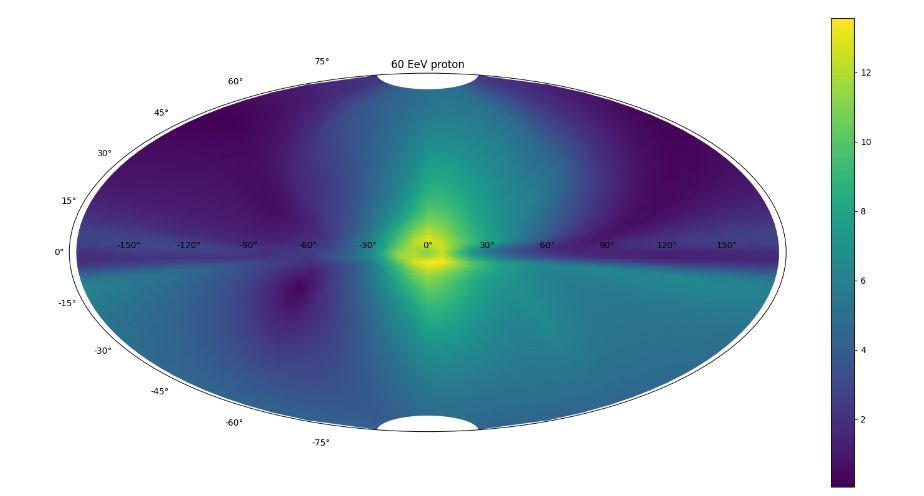
Consider a task of calculation of deflections angles of the 60 EeV protons in the galactic medium observed from the solar system (SS). To do so we generate numerous amount of protons near the SS and backtrace them into the outskirts of the galaxy (28.5 kpc from the SS).

To give that kind of break condition, we define the R_max-the maxium distance, and BCcenter - the point relative which R_max is calulated.

BreakConditions = [{'Rmax': 28.5*Units.kpc}, np.array([-8.5, 0, 0])*Units.kpc]

The trajectories are calculated in JF12mod field, without and distrubances in the field (as energy is too high and particles’ diffusion is small).

Bfield = JF12mod(use_noise = False)

We define the Flux parameter to initialize particles. Unlike the example in the Magnetosphere example the backtracking is achieved with “Mode”: “Outward”, while there we used ForwardTrck=-1. Nevertheless the two methods are equivalent.

InitialFlux =  Flux(Spectrum = Monolines(energy=60e3*Units.PeV),
                    Distribution = SphereSurf(Center = np.array([-8.5,  0. ,  0. ])*Units.kpc, Radius=0),
                    Nevents= 100,
                    Mode = 'Outward',
                    Names = 'pr')

import os
import argparse

import numpy as np
from datetime import datetime

from gtsimulation.Global import Regions, Units
from gtsimulation.Algos import BunemanBorisSimulator
from gtsimulation.Particle import Flux
from gtsimulation.Particle.Generators import Monolines, SphereSurf
from gtsimulation.MagneticFields.Galaxy import JF12mod

parser = argparse.ArgumentParser()
parser.add_argument("--folder")
parser.add_argument("--seed", type=int)

args = parser.parse_args()
folder = args.folder
seed = args.seed
R = args.R

np.random.seed(seed)
Region = Regions.Galaxy
Bfield = JF12mod(use_noise = False)

Date = datetime(2008, 1, 1)

Medium = None
InitialFlux =  Flux(Spectrum = Monolines(energy=60e3*Units.PeV),
                    Distribution = SphereSurf(Center = np.array([-8.5,  0. ,  0. ])*Units.kpc, Radius=0),
                    Nevents= 100,
                    Mode = 'Outward',
                    Names = 'pr')
UseDecay = False
NuclearInteraction = None


Nfiles = 100
Output = f"{folder}" + os.sep + "Dir"
Save = [1000, {"Angles": True, "Clock": True}]

Verbose = True

BreakConditions = [{'Rmax': 28.5*Units.kpc}, np.array([-8.5, 0, 0])*Units.kpc]

simulator = BunemanBorisSimulator(Date=Date, Region=Region, Bfield=Bfield, Medium=Medium, Particles=InitialFlux, Num=int(100000000),
                                Step=1000000, Save=Save, Nfiles=Nfiles, Output=Output, Verbose=Verbose, UseDecay=UseDecay,
                                InteractNUC=NuclearInteraction, BreakCondition=BreakConditions)
simulator()

By calculting the \(\arccos\frac{\vec{v}_0\cdot(\vec{r}_f - \vec{r}_i)}{|\vec{r}_f - \vec{r}_i|}\), we find the deflection angle. Here \(\vec{v}_0\) is the normalized initial velocity, \(\vec{r}_f\) and \(\vec{r}_i\) are final and inital coordinates respectively. The image shows the deflection angles depenadacne from the direction, the color corresponds to the angle in degress.