Backtracing
This notebook demonstrates trajectory tracing and backtracing in GT simulation by integrating the relativistic equation of motion of a charged particle in a prescribed magnetic field.
To make the test fully controlled, the magnetic field is chosen to be uniform, so the expected motion is a helix with a known analytical solution. We compute:
a forward-traced trajectory (normal time direction),
a backward-traced trajectory (reverse time direction), and compare both with the analytical helix.
Expected output:
3D and 2D (XY) plots showing forward, backward, and analytical trajectories.
A diagnostic plot quantifying the deviation from the analytical solution for both forward and backward integration.
from datetime import datetime

import matplotlib.pyplot as plt
import numpy as np
from gtsimulation.Algos import BunemanBorisSimulator
from gtsimulation.Global import Regions, Constants, Units
from gtsimulation.MagneticFields import Uniform
from gtsimulation.Particle import Generators, Flux
Forward tracing (reference trajectory)
This section runs a standard forward trajectory integration:
create one proton with mono-energetic spectrum and a user-defined initial position/velocity,
run the Buneman–Boris integrator with
ForwardTrck=1,extract the computed coordinates and velocities along the track.
Expected output: arrays r_forward and v_forward describing the forward-traced helical trajectory in a uniform magnetic field.
particle_forward = Flux(
    Spectrum=Generators.Spectrums.Monolines(energy=T * Units.MeV),
    Distribution=Generators.Distributions.UserInput(
        R0=[14.542, 0, 0],
        V0=v_0
    ),
    Names="proton",
    Nevents=1
)
simulator_forward = BunemanBorisSimulator(
    Bfield=b_field,
    Region=region,
    Medium=medium,
    Particles=particle_forward,
    InteractNUC=nuclear_interaction,
    UseDecay=use_decay,
    Date=date,
    Step=dt,
    Num=n_steps,
    ForwardTrck=1,
    BreakCondition=break_conditions,
    Save=save,
    Output=output,
    Verbose=verbose
)
track_forward = simulator_forward()[0][0]
Creating simulator object...
Date: 2008-01-01 00:00:00
Time step: 1e-09 seconds
Number of steps: 3000
Radiation Losses: False
Synchrotron Emission: False
Region: Undefined
		Additional Energy Losses: False
Number of files: 1
Output file name: None_num.npy
Save every 1 step of:
	Coordinates: True
	Velocities: True
	Efield: False
	Bfield: False
	Angles: False
	Path: False
	Density: False
	Clock: False
	Energy: False
	PitchAngles: False
	LarmorRadii: False
	GuidingCenter: False
Electric field: None
Magnetic field: Uniform
            B: [0.e+00 0.e+00 1.e+08] nT
Medium: None
Decay: False
Nuclear Interactions: None
Flux:
        Number of particles: 1
        Particles: ['proton']
        V: Isotropic
        Spectrum: Monolines
        Energy: 100
        Distribution: User Input
        R0 shape: (1, 3)
        V0 shape: (1, 3)
Break Conditions:
	Xmin: 0.0
	Ymin: 0.0
	Zmin: 0.0
	Rmin: 0.0
	Dist2Path: 0.0
	Xmax: inf
	Ymax: inf
	Zmax: inf
	Rmax: inf
	MaxPath: inf
	MaxTime: inf
	MaxRev: inf
	Death: inf
BC center: [0 0 0]
Simulator object created!

Launching simulation...

File 1/1 started

Event 1/1 started
Particle: proton (M = 938.272088 [MeV/c2], Z = 1)
Energy: 100.000000 [MeV], Rigidity: 0.444583 [GV]
Coordinates: [14.542  0.     0.   ] [m]
Velocity: [ 0.         -0.98058068  0.19611614]
Beta: 0.4281954849788152
Beta * dt: 0.128370 [m]
Calculating:
	Progress: 0%
	Progress: 10%
	Progress: 20%
	Progress: 30%
	Progress: 40%
	Progress: 50%
	Progress: 60%
	Progress: 70%
	Progress: 80%
	Progress: 90%
	Progress: 100%
Event 1/1 finished in 2.088 seconds

Simulation completed!
r_forward = track_forward["Track"]["Coordinates"]
v_forward = track_forward["Track"]["Velocities"]
Backward tracing (time-reversal check)
This section demonstrates backtracing by integrating the trajectory in the reverse time direction:
use the last point of the forward trajectory as the starting state (position and velocity),
run the same integrator with
ForwardTrck=-1,record the backward-traced coordinates.
Expected output: r_backward should retrace the forward solution (up to numerical error), illustrating time-reversal consistency of the tracing setup.
particle_backward = Flux(
    Spectrum=Generators.Spectrums.Monolines(energy=T * Units.MeV),
    Distribution=Generators.Distributions.UserInput(
        R0=r_forward[-1, :],
        V0=v_forward[-1, :]
    ),
    Names="proton",
    Nevents=1
)
simulator_backward = BunemanBorisSimulator(
    Bfield=b_field,
    Region=region,
    Medium=medium,
    Particles=particle_backward,
    InteractNUC=nuclear_interaction,
    UseDecay=use_decay,
    Date=date,
    Step=dt,
    Num=n_steps,
    ForwardTrck=-1,
    BreakCondition=break_conditions,
    Save=save,
    Output=output,
    Verbose=verbose
)
track_backward = simulator_backward()[0][0]
Creating simulator object...
Date: 2008-01-01 00:00:00
Time step: 1e-09 seconds
Number of steps: 3000
Radiation Losses: False
Synchrotron Emission: False
Region: Undefined
		Additional Energy Losses: False
Number of files: 1
Output file name: None_num.npy
Save every 1 step of:
	Coordinates: True
	Velocities: True
	Efield: False
	Bfield: False
	Angles: False
	Path: False
	Density: False
	Clock: False
	Energy: False
	PitchAngles: False
	LarmorRadii: False
	GuidingCenter: False
Electric field: None
Magnetic field: Uniform
            B: [0.e+00 0.e+00 1.e+08] nT
Medium: None
Decay: False
Nuclear Interactions: None
Flux:
        Number of particles: 1
        Particles: ['proton']
        V: Isotropic
        Spectrum: Monolines
        Energy: 100
        Distribution: User Input
        R0 shape: (1, 3)
        V0 shape: (1, 3)
Break Conditions:
	Xmin: 0.0
	Ymin: 0.0
	Zmin: 0.0
	Rmin: 0.0
	Dist2Path: 0.0
	Xmax: inf
	Ymax: inf
	Zmax: inf
	Rmax: inf
	MaxPath: inf
	MaxTime: inf
	MaxRev: inf
	Death: inf
BC center: [0 0 0]
Simulator object created!

Launching simulation...

File 1/1 started

Event 1/1 started
Backtracing mode is ON
Redefinition of particle to antiparticle
Particle: anti_proton (M = 938.272088 [MeV/c2], Z = -1)
Energy: 100.000000 [MeV], Rigidity: -0.444583 [GV]
Coordinates: [  9.79592579 -10.68462308  75.50097819] [m]
Velocity: [ 0.72186399  0.66366471 -0.19611614]
Beta: 0.4281954849788152
Beta * dt: 0.128370 [m]
Calculating:
	Progress: 0%
	Progress: 10%
	Progress: 20%
	Progress: 30%
	Progress: 40%
	Progress: 50%
	Progress: 60%
	Progress: 70%
	Progress: 80%
	Progress: 90%
	Progress: 100%
Event 1/1 finished in 0.045 seconds

Simulation completed!
r_backward = track_backward["Track"]["Coordinates"]
Analytical helix in a uniform magnetic field
In a uniform magnetic field, the expected motion is a helix:
circular gyromotion in the plane perpendicular to B with cyclotron frequency,
constant motion along B.
This block computes an analytical reference trajectory r_analytic using the chosen field strength and particle energy, so it can be compared directly to the numerically integrated forward/backward tracks.
Expected output: an array r_analytic of the same length as the simulated tracks.
m_p = 938.27  # proton mass [MeV/c²]
gamma = (m_p + T) / m_p
omega = Constants.e * B / (gamma * m_p * Units.MeV2kg)  # cyclotron frequency [Hz]

_, v_y, v_z = Constants.c * np.sqrt(1 - 1 / gamma ** 2) * v_0
r_larmor = gamma * m_p * Units.MeV2kg * np.abs(v_y) / (Constants.e * B)

t = np.linspace(0, dt * n_steps, n_steps)
x = r_larmor * np.cos(omega * t)
y = -r_larmor * np.sin(omega * t)
z = v_z * t

r_analytic = np.stack((x, y, z), axis=1)
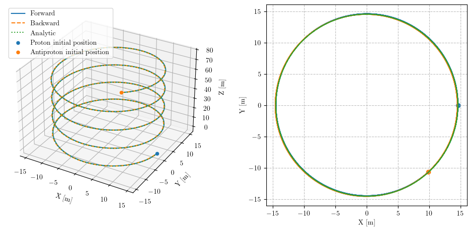
Visual comparison: forward vs backward vs analytic
This block overlays three trajectories:
forward-traced (solid),
backward-traced (dashed),
analytical reference (dotted).
Expected output:
a 3D plot showing the helix geometry and the consistency between all three curves,
an XY-plane projection highlighting the circular gyromotion and the agreement between numerical and analytical solutions.
fig = plt.figure(figsize=(12, 6))

ax3d = fig.add_subplot(1, 2, 1, projection='3d')

ax3d.plot(*r_forward.T, label="Forward")
ax3d.plot(*r_backward.T, label="Backward", linestyle="--")
ax3d.plot(*r_analytic.T, label="Analytic", linestyle=":")

ax3d.scatter(*r_forward[0], label='Proton initial position')
ax3d.scatter(*r_backward[0], label="Antiproton initial position")

ax3d.set_xlabel("X [m]")
ax3d.set_ylabel("Y [m]")
ax3d.set_zlabel("Z [m]")
ax3d.set_aspect('equalxy')
ax3d.legend()

ax2d = fig.add_subplot(1, 2, 2)

ax2d.plot(*r_forward.T[:2], label="Forward")
ax2d.plot(*r_backward.T[:2], label="Backward", linestyle="--")
ax2d.plot(*r_analytic.T[:2], label="Analytic", linestyle=":")

ax2d.scatter(*r_forward[0][:2])
ax2d.scatter(*r_backward[0][:2])

ax2d.set_xlabel("X [m]")
ax2d.set_ylabel("Y [m]")
ax2d.set_aspect('equal')
ax2d.grid(True, linestyle='--', alpha=0.8)

fig.subplots_adjust(wspace=0.3)

plt.show()
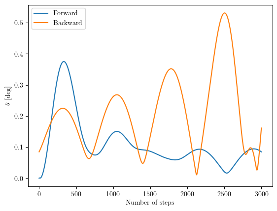
Deviation from the analytical solution
This section quantifies how well the numerical integration matches the analytical helix:
compute an angle-like phase mismatch for the forward track relative to
r_analytic,compute the analogous mismatch for the backward track relative to the time-reversed analytical curve (
r_analytic[::-1]),plot both mismatch curves versus step index.
Expected output: a diagnostic plot where both forward and backward deviations remain small (and typically grow slowly with step count due to numerical error accumulation).
# Forward trajectory
dot_forward = np.sum(r_forward * r_analytic, axis=1)
norm_forward = np.linalg.norm(r_forward, axis=1) * np.linalg.norm(r_analytic, axis=1)
phase_forward = np.rad2deg(np.arccos(dot_forward / norm_forward))

# Backward trajectory
dot_backward = np.sum(r_backward * r_analytic[::-1], axis=1)
norm_backward = np.linalg.norm(r_backward, axis=1) * np.linalg.norm(r_analytic[::-1], axis=1)
phase_backward = np.rad2deg(np.arccos(dot_backward / norm_backward))
fig = plt.figure()
ax = fig.subplots()

ax.plot(phase_forward, label="Forward")
ax.plot(phase_backward, label="Backward")

ax.set_xlabel("Number of steps")
ax.set_ylabel(r"$\theta$ [deg]")
ax.legend()

plt.show()