Deflection in Galaxy

This notebook demonstrates the simulation of Ultra-High-Energy Cosmic Ray (UHECR) propagation through the Galaxy. The goal is to estimate the deflection of protons with energies \(E = 60~\text{EeV}\) caused by the Galactic magnetic field (GMF).

At such high energies (\(> 10^{18}\) eV), the Larmor radius of particles becomes comparable to the size of the Galaxy, and diffusion effects are negligible. Therefore, we can simulate their propagation using trajectory backtracing:

• Launch antiparticles (antiprotons) from the Solar System in various directions covering the celestial sphere.

• Trace them through the GMF model (Jansson & Farrar, JF12) until they escape the Galactic halo.

• Calculate the angle between the initial launch direction and the final position vector.

The deflection angle \(\alpha\) is calculated as:

\[ \alpha = \arccos\left( \frac{\mathbf{v}_0 \cdot (\mathbf{r}_f - \mathbf{r}_0)}{|\mathbf{r}_f - \mathbf{r}_0|}\right) \]

where:

• \(\mathbf{v}_0\) is the initial normalized velocity vector (direction of observation),

• \(\mathbf{r}_0\) is the starting position (Solar System),

• \(\mathbf{r}_f\) is the final position where the particle escapes the Galaxy.

Expected Output:

A sky map (Galactic coordinates) showing the magnitude of deflection for 60 EeV protons, highlighting the anisotropic influence of the large-scale magnetic field structure.

from datetime import datetime

import matplotlib.pyplot as plt
import numpy as np
from gtsimulation.Algos import BunemanBorisSimulator
from gtsimulation.Global import Regions, Units
from gtsimulation.MagneticFields.Galaxy import JF12mod
from gtsimulation.Particle import Generators, Flux

Simulation settings

We define the global simulation environment:

• Magnetic Field: Jansson & Farrar (2012) model (JF12), random component disabled (use_noise=False) to study the regular field effect.

• Region: Galaxy.

• Time Step: Large step (\(1000\) days) is sufficient for UHECRs due to their immense rigidity.

• Break Conditions: Simulation stops when the particle reaches the Galactic halo boundary (\(R > 28.5\) kpc).

date = datetime(2025, 1, 1)
region = Regions.Galaxy
b_field = JF12mod(use_noise=False)
medium = None

use_decay = False
nuclear_interaction = None

dt = 1000 * Units.day  # time step [s]
n_steps = int(1e5)

# dt = 100 * Units.day  # time step [s]
# n_steps = int(1e6)

break_conditions = [{"Rmax": 28.5 * Units.kpc}, np.array([-8.5, 0, 0]) * Units.kpc]

save = [0, {"Coordinates": True, "Velocities": True}]
output = None

verbose = 0

The function get_deflection_angle performs the core logic for a single direction \((l, b)\):

• Converts Galactic coordinates \((l, b)\) to a velocity vector.

• Initializes an anti-proton at the Solar System location \((-8.5, 0, 0)\) kpc.

• Runs the BunemanBorisSimulator.

• Computes the deflection angle \(\alpha\) using the formula defined in the introduction.

def get_deflection_angle(l, b):
    v = np.array([
        np.cos(np.deg2rad(l)) * np.cos(np.deg2rad(b)),
        np.sin(np.deg2rad(l)) * np.cos(np.deg2rad(b)),
        np.sin(np.deg2rad(b))
    ])
    particle = Flux(
        Spectrum=Generators.Spectrums.UserInput(energy=60 * Units.EeV),
        Distribution=Generators.Distributions.UserInput(
            R0=np.array([-8.5, 0, 0]) * Units.kpc,
            V0=v
        ),
        Names="anti_proton"
    )
    simulator = BunemanBorisSimulator(
        Bfield=b_field,
        Region=region,
        Medium=medium,
        Particles=particle,
        InteractNUC=nuclear_interaction,
        UseDecay=use_decay,
        Date=date,
        Step=dt,
        Num=n_steps,
        BreakCondition=break_conditions,
        Save=save,
        Output=output,
        Verbose=verbose
    )
    event = simulator()[0][0]
    r_0 = event['Particle']['R0']
    r_f = event['Track']['Coordinates'][-1]
    v_0 = event['Particle']['V0']
    angle = np.acos(np.dot(v_0, (r_f - r_0)) / np.linalg.norm(r_f - r_0))
    return np.rad2deg(angle)

Global scan setup

We define a grid in Galactic coordinates \((l, b)\) to map the deflection angles across the entire sky.

• Longitude \(l\): -180 to 180 degrees.

• Latitude \(b\): -90 to 90 degrees.

from joblib import Parallel, delayed
from tqdm_joblib import tqdm_joblib

from mpl_toolkits.axes_grid1 import make_axes_locatable

/home/rustam/Документы/МИФИческое/научка/software/GTsimulation/.venv/lib/python3.12/site-packages/tqdm_joblib/__init__.py:4: TqdmExperimentalWarning: Using `tqdm.autonotebook.tqdm` in notebook mode. Use `tqdm.tqdm` instead to force console mode (e.g. in jupyter console)
  from tqdm.autonotebook import tqdm

l_grid = np.arange(-180, 180, 10)
b_grid = np.arange(-90, 91, 10)
a_grid = np.empty((b_grid.size, l_grid.size))

Since each direction is independent, we use joblib to parallelize the computation across all available CPU cores.

def worker(i_l, i_b):
    angle = get_deflection_angle(l_grid[i_l], b_grid[i_b])
    return i_l, i_b, angle

tasks = [(i, j) for i in range(l_grid.size) for j in range(b_grid.size)]
with tqdm_joblib(total=len(tasks)):
    res = Parallel(n_jobs=-1)(delayed(worker)(i, j) for i, j in tasks)
for i_l, i_b, v in res:
    a_grid[i_b, i_l] = v

# add the 180° meridian and copy values from the -180° meridian in order to stitch the map seamlessly
l_grid = np.hstack((l_grid, 180))
a_grid = np.pad(a_grid, pad_width=((0, 0), (0, 1)), mode="wrap")

Visualization

We present the results in two formats:

• Rectangular Projection: Useful for inspecting the raw data grid.

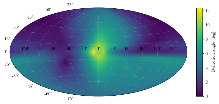
• Mollweide/Aitoff Projection: Standard astronomical projection for full-sky maps.

fig = plt.figure(figsize=(8, 4))
ax = fig.subplots()

pcm = ax.pcolormesh(l_grid, b_grid, a_grid, vmin=0)
ax.set_xlim(-180, 180)
ax.set_ylim(-90, 90)

ax.set_xticks(np.arange(-180, 181, 60))
ax.set_yticks(np.arange(-90, 91, 30))
ax.set_xlabel('Galactic longitude [deg]')
ax.set_ylabel('Galactic latitude [deg]')

divider = make_axes_locatable(ax)
cax = divider.append_axes("right", size="3.5%", pad=0.3, axes_class=plt.Axes)
fig.colorbar(pcm, cax=cax, label="Deflection angle [deg]")

plt.show()

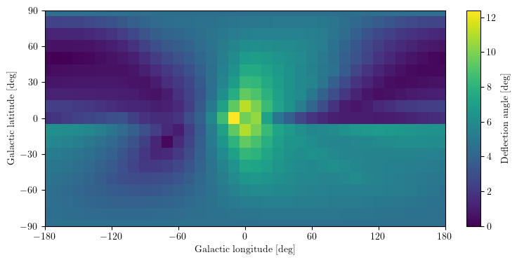
fig = plt.figure(figsize=(8, 4))
ax = fig.add_subplot(111, projection="aitoff")

pcm = ax.pcolormesh(np.deg2rad(l_grid), np.deg2rad(b_grid), a_grid, shading="gouraud", vmin=0)
ax.grid(True, linestyle=':', alpha=0.5)

divider = make_axes_locatable(ax)
cax = divider.append_axes("right", size="3.5%", pad=0.3, axes_class=plt.Axes)
fig.colorbar(pcm, cax=cax, label="Deflection angle [deg]")

plt.show()

# fig.savefig("deflection_angles.pdf")

The resulting map shows the anisotropic nature of UHECR deflection.

• Galactic Plane (\(b \approx 0\)): Higher deflection angles are typically observed due to the stronger magnetic fields in the Galactic disk.

• High Latitudes: Deflections are generally smaller.

Potential ways to improve accuracy:

• Decrease the integration time step (e.g., down to 1 day).

• Increase the latitude/longitude grid resolution.