Interaction probability
This notebook demonstrates the verification of the nuclear interaction module in the GT simulation package.
The goal is to simulate the propagation of cosmic ray protons through the interstellar medium (ISM) and calculate the probability of inelastic nuclear interactions as a function of energy.
The interaction probability is governed by an exponential attenuation law. For a particle traversing a grammage \(X\) (column density of matter in g/cm\(^2\)), the probability of undergoing an inelastic collision is given by:
Workflow overview:
Define the ISM properties (homogeneous hydrogen gas) and the primary particle spectrum (protons, 1 GeV – 1 TeV, log-uniform distribution).
For each particle, assign a target path length (grammage \(X\)) based on the empirical Path Length Distribution.
Trace particles through the medium until they either interact or pass the assigned grammage.
Calculate the fraction of interacting particles in energy bins.
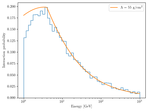
Compare the simulated interaction probability with the theoretical expectation for \(\Lambda = 55 \text{ g/cm}^2\).
Expected output: A plot showing the interaction probability vs. energy, where simulation data points should align with the theoretical curve, confirming the correct implementation of the physics module.
import numpy as np
import matplotlib.pyplot as plt

from gtsimulation.Global import Units
Path length distribution (grammage)
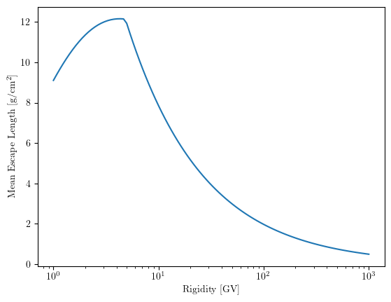
We use a parameterized function to represent the mean escape length (grammage) traversed by cosmic rays in the Galaxy as a function of their rigidity \(R\). This distribution corresponds to the “Nested Leaky Box” model or similar empirical fits (e.g., Simon et al., 1998).
The function below calculates the grammage \(X(R)\) in g/cm\(^2\).
def grammage(R, Rb=4.8362, coeffs=(2.2089, 0.4517, -0.2111, 0.0256), k=-0.6):
    a, b, c, d = coeffs
    ln_xb = np.log(Rb)
    A2 = np.exp(a + b*ln_xb + c*ln_xb**2 + d*ln_xb**3) / (Rb**k)
    return np.piecewise(R, [R <= Rb, R > Rb], [
        lambda t: np.exp(a + b*np.log(t) + c*np.log(t)**2 + d*np.log(t)**3),
        lambda t: A2 * t**k
    ])
R_line = np.geomspace(1, 1e3, 100)

fig = plt.figure()
ax = fig.subplots()

ax.plot(R_line, grammage(R_line))
ax.set_xlabel("Rigidity [GV]")
ax.set_ylabel("Mean Escape Length [g/cm$^2$]")
ax.set_xscale("log")

plt.show()
Simulation settings
Here we define the initial conditions and physical parameters:
Particles \(10^5\) protons.
Energy Range 1 GeV to 1 TeV.
Medium: Interstellar hydrogen gas with number density \(n = 1 \text{ cm}^{-3}\).
T_min = 1 * Units.GeV
T_max = 1 * Units.TeV

n_events = 100_000

pdg_code = 2212 # proton
n_ism = 1       # interstellar hydrogen gas density [cm^-3]
m_H = 1.66e-24  # hydrogen mass [g]
rho_ism = n_ism * m_H # mass density [g cm^-3]
We generate a sample of primary protons with energies distributed log-uniformly. For each proton, we calculate its rigidity \(R\) and assign a corresponding grammage \(X(R)\) that it attempts to traverse.
def log_uniform(a, b, size=None):
    log_samples = np.random.uniform(np.log(a), np.log(b), size)
    return np.exp(log_samples)
T_range = log_uniform(T_min, T_max, n_events)
R_range = np.sqrt((T_range / Units.GeV + 0.93827) ** 2 - 0.93827 ** 2) # rigidity [GV]
X_range = grammage(R_range)
Running the simulation
We use ProcessPoolExecutor to parallelize the simulation.
The dataset is split into n_tasks chunks. Each task simulates the transport of a batch of protons through the matter layer.
Note: The process_chunk_safe function runs the interaction module for each particle. It returns a boolean flag indicating whether an interaction occurred (True) or the particle passed through without interaction (False).
from concurrent.futures import ProcessPoolExecutor, as_completed
from tqdm import tqdm

n_tasks = 20
T_chunks = np.array_split(T_range, n_tasks)
X_chunks = np.array_split(X_range, n_tasks)
seeds = range(n_tasks)

def process_chunk_safe(T_chunk, X_chunk, i_task):
    from gtsimulation.Interaction import NuclearInteraction
    sim = NuclearInteraction(seed=i_task)
    interaction_flag = np.zeros(T_chunk.size, dtype=np.bool)
    for i in range(T_chunk.size):
        primary, secondary = sim.run_matter_layer(
            pdg=pdg_code,
            energy=T_chunk[i],
            mass=X_chunk[i],
            density=rho_ism,
            element_name=['H'],
            element_abundance=[1.0]
        )
        interaction_flag[i] = (len(secondary) > 0)
    del sim
    return (i_task, interaction_flag)

with ProcessPoolExecutor() as executor:
    futures = [
        executor.submit(process_chunk_safe, t, x, s)
        for t, x, s in zip(T_chunks, X_chunks, seeds)
    ]
    results = []
    for f in tqdm(as_completed(futures), total=len(futures)):
        results.append(f.result())
100%|███████████████████████████████████████████████████████████████████████████████████████████████████████████████████████████████████████████████████| 20/20 [00:33<00:00, 1.67s/it]
The results arrive out of order due to parallel processing. We sort them by task index to ensure they match the original energy array T_range.
interaction_flag = np.hstack([item[1] for item in sorted(results, key=lambda x: x[0])])
Analysis and Visualization
We compute the interaction probability as the ratio of interacting particles to the total number of particles in logarithmic energy bins.
bins = np.geomspace(T_min, T_max, 50) / Units.GeV

interaction_count, _ = np.histogram(T_range / Units.GeV, bins=bins, weights=interaction_flag.astype('float'))
total_count, _ = np.histogram(T_range / Units.GeV, bins=bins)

interaction_fraction = np.divide(
    interaction_count,
    total_count,
    out=np.zeros_like(interaction_count),
    where=total_count != 0
)
Finally, we plot the simulated data against the theoretical prediction for a constant nuclear interaction length \(\Lambda = 55 \text{ g/cm}^2\).
fig = plt.figure()
ax = fig.subplots()

ax.stairs(interaction_fraction, bins)

L = 55 # nuclear interaction length [g cm^-2]
T_line = np.geomspace(T_min, T_max, 100)
R_line = np.sqrt((T_line / Units.GeV + 0.93827) ** 2 - 0.93827 ** 2) # rigidity [GV]
ax.plot(T_line / Units.GeV, 1 - np.exp(-grammage(R_line) / L),
        label=rf'$\Lambda$ = {L} g/cm$^2$')

ax.set_xscale('log')
ax.set_xlabel('Energy [GeV]')
ax.set_ylabel('Interaction probability')
ax.legend()

plt.show()