Motion in dipole magnetic field

This notebook demonstrates a basic GT simulation workflow for numerically integrating the equation of motion of a charged particle in the Earth’s magnetic field approximated by a dipole model.

Goals of this example:

• Define the Dipole magnetic field and initial conditions for a single particle (a 10 MeV proton).

• Compute the trajectory with two integrators: Buneman–Boris (BB) and 6th‑order Runge–Kutta (RK6).

• Visually compare trajectories in the XY plane and estimate a characteristic cyclotron motion scale (the Larmor radius) along the trajectory.

Expected output:

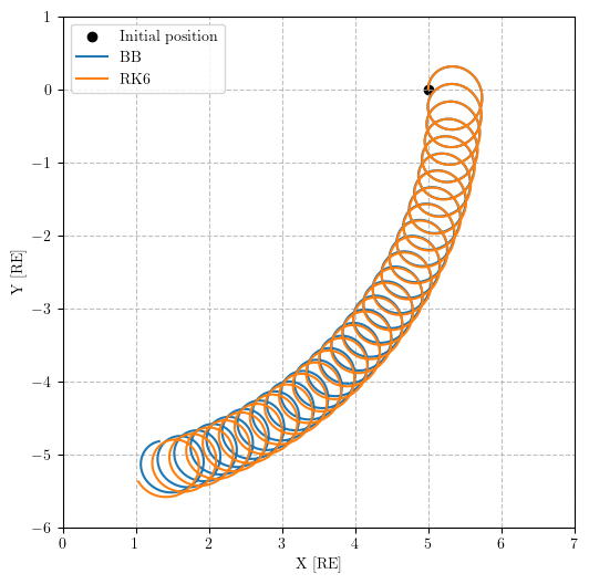
• A plot of BB and RK6 trajectories starting from the same point and showing the difference in the results of calculations using two numerical schemes for a selected time step.

• A plot of the Larmor radius versus step index (for both methods), including the minimum/maximum (R_L) over the simulated interval.

from datetime import datetime

import matplotlib.pyplot as plt
import numpy as np
from gtsimulation.Algos import BunemanBorisSimulator, RungeKutta6Simulator
from gtsimulation.Global import Regions, Units
from gtsimulation.MagneticFields.Magnetosphere import Dipole
from gtsimulation.Particle import Generators, Flux

Problem setup: field, particle, and integration parameters

This section defines the simulation setup:

• date (used by time-dependent field models);

• the Magnetosphere region and the Dipole field model;

• particle initial conditions: a single 10 MeV proton starting at ([5 R_E, 0, 0]) point in the geocentric coordinate system (also known as ECEF) with an initial velocity directed along (Y) axis;

• integration settings: total simulated time total_time, number of steps n_steps, and time step dt;

• which quantities to store in the track (coordinates, velocities, energy, and magnetic field values along the trajectory).

The expected outcome of this block is a fully defined configuration that can be passed to different numerical schemes for comparison.

date = datetime(2008, 1, 1)
region = Regions.Magnetosphere
b_field = Dipole(date=date)
medium = None

particle = Flux(
    Spectrum=Generators.Spectrums.Monolines(energy=10 * Units.MeV),
    Distribution=Generators.Distributions.UserInput(
        R0=np.array([5 * Units.RE, 0, 0]),
        V0=[0, 1, 0]
    ),
    Names="proton",
    Nevents=1
)

use_decay = False
nuclear_interaction = None

total_time = 10  # total time [s]
n_steps = 20000
dt = total_time / n_steps
break_conditions = None

save = [1, {"Coordinates": True, "Velocities": True, "Energy": True, "Bfield": True}]
output = None

verbose = 0

Trajectory computation: Buneman–Boris (BB) scheme

This block creates a BunemanBorisSimulator instance and runs the particle trajectory calculation in the given magnetic field.

After execution, the following arrays are extracted:

• r_BB — trajectory coordinates,

• v_BB — velocities,

• T_BB — particle energy along the trajectory,

• B_BB — magnetic field sampled at trajectory points.

The output arrays of coordinate, velocity and field vectors are also expressed in the geocentric coordinate system.

The expected result is a stable trajectory (BB is a common choice for particle tracing in electromagnetic fields) and a dataset suitable for comparison with other integrators.

simulator_BB = BunemanBorisSimulator(
    Bfield=b_field,
    Region=region,
    Medium=medium,
    Particles=particle,
    InteractNUC=nuclear_interaction,
    UseDecay=use_decay,
    Date=date,
    Step=dt,
    Num=n_steps,
    BreakCondition=break_conditions,
    Save=save,
    Output=output,
    Verbose=verbose
)

track_BB = simulator_BB()[0][0]
r_BB = track_BB["Track"]["Coordinates"]
v_BB = track_BB["Track"]["Velocities"]
T_BB = track_BB["Track"]["Energy"]
B_BB = track_BB["Track"]["Bfield"]

Trajectory computation: 6th-order Runge–Kutta (RK6)

This block repeats the same calculation for the same initial conditions, but using the RungeKutta6Simulator integrator.

After execution, the arrays

• r_RK6, v_RK6, T_RK6, B_RK6 are obtained analogously to the BB case.

The expected result is that the RK6 trajectory closely matches the BB trajectory for a sufficiently small dt, with possible small differences due to method properties and numerical error accumulation.

simulator_RK6 = RungeKutta6Simulator(
    Bfield=b_field,
    Region=region,
    Medium=medium,
    Particles=particle,
    InteractNUC=nuclear_interaction,
    UseDecay=use_decay,
    Date=date,
    Step=dt,
    Num=n_steps,
    BreakCondition=break_conditions,
    Save=save,
    Output=output,
    Verbose=verbose
)

track_RK6 = simulator_RK6()[0][0]
r_RK6 = track_RK6["Track"]["Coordinates"]
v_RK6 = track_RK6["Track"]["Velocities"]
T_RK6 = track_RK6["Track"]["Energy"]
B_RK6 = track_RK6["Track"]["Bfield"]

Trajectory comparison (BB vs RK6)

This section plots the trajectories in the XY plane (in Earth radii (R_E)):

• the starting point is marked explicitly;

• trajectories computed with BB and RK6 are overlaid.

The expected output is a clear visual comparison of the trajectories calculated using the two numerical schemes. At the chosen time step dt, discrepancies in the trajectories become visible, and these discrepancies accumulate.

fig = plt.figure(figsize=(6, 6))
ax = fig.subplots()

ax.scatter(5, 0, label="Initial position", color="black")
ax.plot(*r_BB.T[:2] / Units.RE, label="BB")
ax.plot(*r_RK6.T[:2] / Units.RE, label="RK6")

ax.set_xlim(0, 7)
ax.set_ylim(-6, 1)
ax.set_xlabel("X [RE]")
ax.set_ylabel("Y [RE]")
ax.set_aspect("equal")
ax.grid(True, linestyle="--", alpha=0.8)
ax.legend()

plt.show()

Estimating the Larmor radius along the trajectory

This section evaluates a characteristic spatial scale of the cyclotron motion—the Larmor radius (R_L)—as a function of time/step index.

Workflow:

• import GetLarmorRadius;

• read particle mass and charge from the simulation output;

• compute the pitch angle (angle between velocity and magnetic-field direction) and then (R_L) at each trajectory point;

• plot (R_L) (in (R_E)) for BB and RK6 and indicate the minimum/maximum values.

The expected output is two close (R_L) curves and an understanding of how the local Larmor radius changes as the particle moves through a non-uniform dipole field.

from gtsimulation.MagneticFields.Magnetosphere.Additions import GetLarmorRadius

M = track_BB["Particle"]["M"]
Z = track_BB["Particle"]["Ze"]

B_unit_BB = B_BB / np.linalg.norm(B_BB, axis=1)[:, None]
v_dot_B_BB = np.sum(v_BB * B_unit_BB, axis=1)
pitch_BB = np.rad2deg(np.arccos(v_dot_B_BB))  # clearly get a pitch angle of 90 degrees
LR_BB = GetLarmorRadius(T_BB, np.linalg.norm(B_BB, axis=1), Z, M * Units.MeV2kg, pitch_BB)

B_unit_RK6 = B_RK6 / np.linalg.norm(B_RK6, axis=1)[:, None]
v_dot_B_RK6 = np.sum(v_RK6 * B_unit_RK6, axis=1)
pitch_RK6 = np.rad2deg(np.arccos(v_dot_B_RK6))  # clearly get a pitch angle of 90 degrees
LR_RK6 = GetLarmorRadius(T_RK6, np.linalg.norm(B_RK6, axis=1), Z, M * Units.MeV2kg, pitch_RK6)

fig = plt.figure(figsize=(9, 3))
ax = fig.subplots()

ax.plot(LR_BB / Units.RE, label="BB")
ax.plot(LR_RK6 / Units.RE, label="RK6")

ax.axhline(y=np.min(LR_BB / Units.RE), linestyle=":")
ax.axhline(y=np.max(LR_BB / Units.RE), linestyle=":")

ax.set_xlabel("Number of steps")
ax.set_ylabel("R$_L$ [RE]")
ax.legend(loc="center left")

plt.show()