Trapped particles
This notebook demonstrates the simulation of a charged particle trapped in Earth’s radiation belts. Charged particles in a dipole-like magnetic field undergo three distinct types of periodic motion:
Gyration around magnetic field lines (fastest).
Bounce motion between magnetic mirror points (medium).
Drift motion around the Earth (slowest).
Associated with these periodic motions are three adiabatic invariants. In this example, we simulate a proton in the IGRF magnetic field and verify the conservation of the first (\(I_1\)) and second (\(I_2\)) invariants over a full drift revolution.
Simulation Setup:
Particle: Proton, 40 MeV.
Location: \(L \approx 1.5\) (Inner Radiation Belt).
Pitch Angle: \(135^\circ\) (ensures the particle is trapped and bounces).
Field Model: IGRF-13.
from datetime import datetime

import matplotlib.pyplot as plt
import numpy as np
from gtsimulation.Algos import BunemanBorisSimulator
from gtsimulation.Global import Regions, Units
from gtsimulation.MagneticFields.Magnetosphere import Gauss
from gtsimulation.Particle import Generators, Flux
Simulation configuration
We define a 40 MeV proton starting at \(1.5 R_E\). The pitch angle \(\alpha\) is defined as the angle between the velocity vector and the magnetic field vector. Here, we set \(\alpha = 135^\circ\), which directs the particle towards the Southern Hemisphere mirror point.
We use a high number of steps (450,000) with a small time step (0.1 ms) to accurately resolve the gyromotion while covering enough time for the particle to drift all the way around the Earth (longitudinal drift).
date = datetime(2008, 1, 1)
region = Regions.Magnetosphere
b_field = Gauss(model="IGRF", version=13, model_type="core", date=date)
medium = None

alpha = np.deg2rad(135)
particle = Flux(
    Spectrum=Generators.Spectrums.Monolines(energy=40 * Units.MeV),
    Distribution=Generators.Distributions.UserInput(
        R0=np.array([1.5 * Units.RE, 0, 0]),
        V0=np.array([np.sin(alpha), 0, np.cos(alpha)])
    ),
    Names="proton",
    Nevents=1
)

use_decay = False
nuclear_interaction = None

dt = 1e-4  # time step [s]
n_steps = 450000  # for a full revolution around the Earth
break_conditions = None

save = [1, {"Coordinates": True, "Energy": True}]
output = None

verbose = True
Simulation
We initialize the BunemanBorisSimulator and pass TrackParams={"Invariants": True}. This instructs the simulator to calculate adiabatic invariants (\(I_1, I_2\), Mirror Points, etc.) on-the-fly during the simulation and store them in the output under ["Additions"].
track_params = {"Invariants": True}

simulator = BunemanBorisSimulator(
    Bfield=b_field,
    Region=region,
    Medium=medium,
    Particles=particle,
    InteractNUC=nuclear_interaction,
    UseDecay=use_decay,
    Date=date,
    Step=dt,
    Num=n_steps,
    BreakCondition=break_conditions,
    Save=save,
    Output=output,
    Verbose=verbose,
    TrackParams=track_params
)

track = simulator()[0][0]
r = track["Track"]["Coordinates"]
File 1/1 started
Event 1/1 finished in 13.291 seconds
Simulation completed!
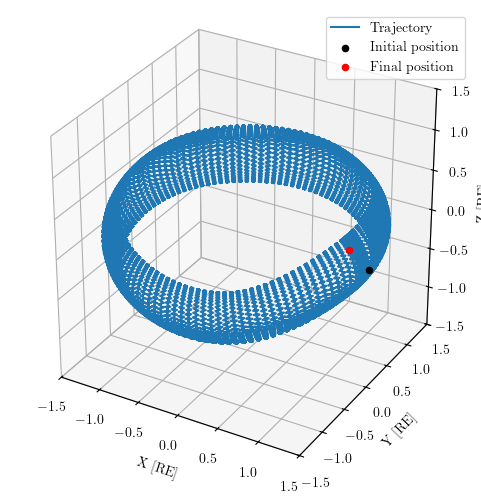
fig = plt.figure(figsize=(7, 6))
ax = fig.add_subplot(projection="3d")

ax.plot(*r.T / Units.RE, label="Trajectory")
ax.scatter(*r[0].T / Units.RE, label="Initial position", color="black")
ax.scatter(*r[-1].T / Units.RE, label="Final position", color="red")

ax.set_xlim(-1.5, 1.5)
ax.set_ylim(-1.5, 1.5)
ax.set_zlim(-1.5, 1.5)
ax.set_xlabel("X [RE]")
ax.set_ylabel("Y [RE]")
ax.set_zlabel("Z [RE]")
ax.set_aspect("equal")
ax.legend()

plt.show()
Analysis of adiabatic invariants
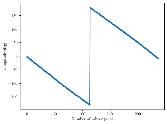
To properly analyze the conservation of invariants during the drift motion, we map the data to the Magnetic Local Time or Longitude. Since the particle bounces between Northern and Southern mirror points, we identify the indices of the “Magnetic Equator” crossings (approximate midpoints between mirror points) to plot the invariants as a function of the drift longitude.
from pyproj import Transformer
i_mirror = track["Additions"]["MirrorPoints"]["NumMirr"]
i_eq = ((i_mirror[:-1] + i_mirror[1:]) / 2).astype(int)
geo_to_lla = Transformer.from_crs(
    {"proj": "geocent", "ellps": "WGS84", "datum": "WGS84"},
    {"proj": "latlong", "ellps": "WGS84", "datum": "WGS84"}
)
lon_eq, _, _ = geo_to_lla.transform(*r[i_eq].T, radians=False)
fig = plt.figure()
ax = fig.subplots()

ax.plot(lon_eq, ".-")
ax.set_xlabel("Number of mirror point")
ax.set_ylabel("Longitude [deg]")

plt.show()
n = len(lon_eq)
area = (lon_eq < 10) & (np.arange(n) < n * 0.66)
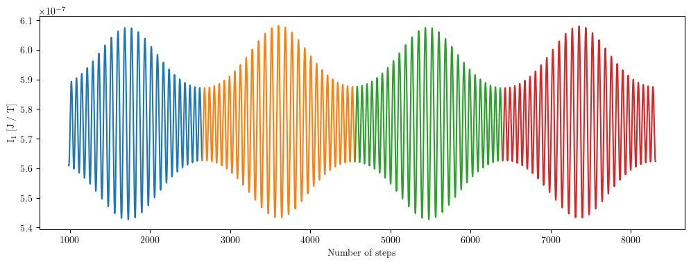
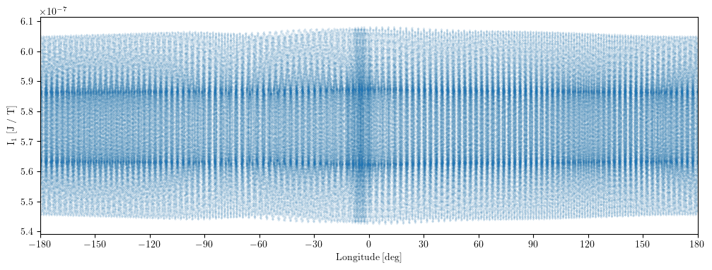
First invariant
The first invariant is associated with the cyclotron motion (gyration) and is defined as the magnetic moment:
Below, we analyze \(I_1\) in two ways:
Instantaneous: Plotting \(I_1\) at every time step for the first few bounces.
Bounce-Averaged: Averaging \(I_1\) over each bounce period and plotting it against longitude for the full revolution.
I1 = track["Additions"]["Invariants"]["I1"]
i_step = np.arange(I1.size)
i_start = i_mirror[:-1]
i_end = i_mirror[1:]

I1_eq = np.array([I1[s:e].mean() for s, e in zip(i_start, i_end)])
I1_eq_mean = np.mean(I1_eq)
fig = plt.figure(figsize=(12, 4))
ax = fig.subplots()

for i in range(4):
    ax.plot(i_step[i_mirror[i]:i_mirror[i + 1]], I1[i_mirror[i]:i_mirror[i + 1]])

ax.set_xlabel("Number of steps")
ax.set_ylabel("I$_1$ [J / T]")

plt.show()
lon, _, _ = geo_to_lla.transform(*r.T, radians=False)

fig = plt.figure(figsize=(12, 4))
ax = fig.subplots()

ax.plot(lon, I1, ".", markersize=0.1)

ax.set_xlim([-180, 180])
ax.set_xlabel("Longitude [deg]")
ax.set_ylabel("I$_1$ [J / T]")

ax.set_xticks(np.arange(-180, 181, 30))

plt.show()
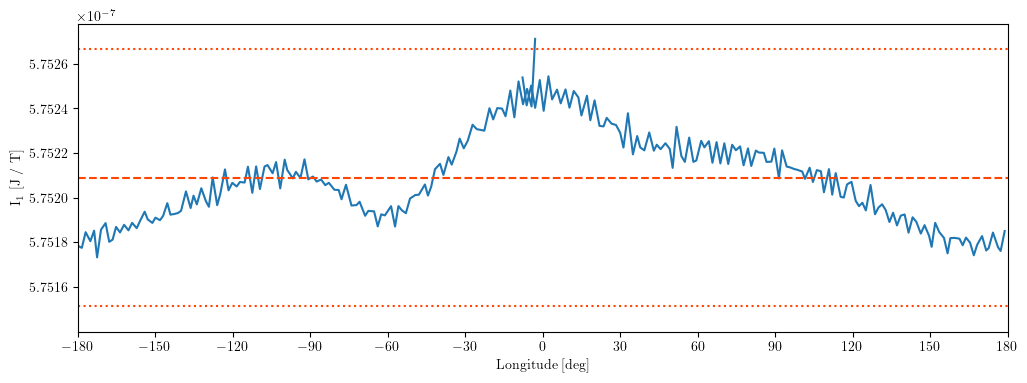
band_width = I1_eq_mean * 0.0001
band_lower = I1_eq_mean - band_width
band_upper = I1_eq_mean + band_width

fig = plt.figure(figsize=(12, 4))
ax = fig.subplots()

ax.plot(lon_eq[area], I1_eq[area], color="tab:blue")
ax.plot(lon_eq[~area], I1_eq[~area], color="tab:blue")

ax.axhline(y=I1_eq_mean, linestyle="--", color="orangered")
ax.axhline(y=band_lower, linestyle=":", color="orangered")
ax.axhline(y=band_upper, linestyle=":", color="orangered")

ax.set_xlim([-180, 180])
ax.set_ylim([band_lower - band_width * 0.2, band_upper + band_width * 0.2])
ax.set_xlabel("Longitude [deg]")
ax.set_ylabel("I$_1$ [J / T]")

ax.set_xticks(np.arange(-180, 181, 30))

plt.show()
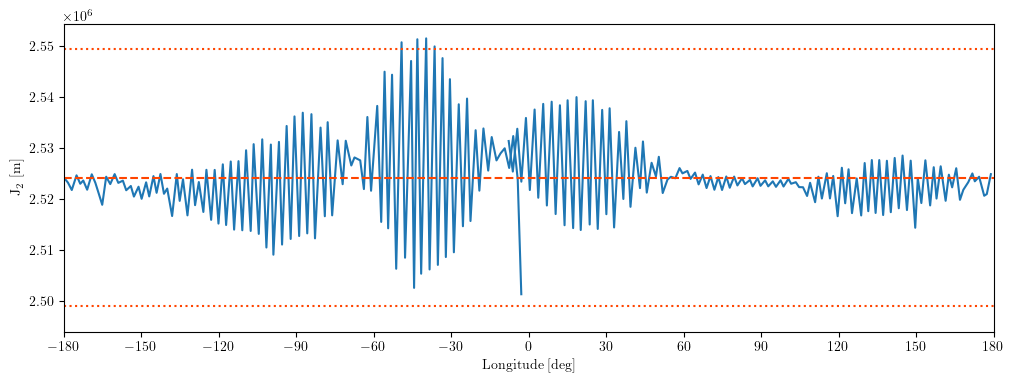
Second invariant
The second invariant is associated with the bounce motion between mirror points and is defined as the integral of the parallel momentum along the field line:
This invariant ensures that as the particle drifts around the Earth, the length of its field line path remains constrained relative to the field strength.
I2 = track["Additions"]["Invariants"]["I2"]
I2_mean = np.mean(I2)
band_width = I2_mean * 0.01
band_lower = I2_mean - band_width
band_upper = I2_mean + band_width

fig = plt.figure(figsize=(12, 4))
ax = fig.subplots()

ax.plot(lon_eq[area], I2[area], color="tab:blue")
ax.plot(lon_eq[~area], I2[~area], color="tab:blue")

ax.axhline(y=I2_mean, linestyle="--", color="orangered")
ax.axhline(y=band_lower, linestyle=":", color="orangered")
ax.axhline(y=band_upper, linestyle=":", color="orangered")

ax.set_xlim([-180, 180])
ax.set_ylim([band_lower - band_width * 0.2, band_upper + band_width * 0.2])
ax.set_xlabel("Longitude [deg]")
ax.set_ylabel("J$_2$ [m]")

ax.set_xticks(np.arange(-180, 181, 30))

plt.show()