Geomagnetic cutoff rigidity
This notebook demonstrates how to compute the vertical geomagnetic cutoff rigidity at a given geographic location by backtracing charged particles through the geomagnetic field.
The key idea is to perform backtracing of charged particles in a realistic geomagnetic field model (IGRF). For a given geographic location and a set of trial rigidities, each trajectory is classified as:
allowed (the particle can reach the location from outside the magnetosphere), or
forbidden (the particle is blocked/trapped and does not reach the location from outside).
This allowed/forbidden pattern as a function of rigidity is often called a cutoff barcode, and the transition region is the penumbra.
Workflow overview:
Define the magnetospheric magnetic field model (IGRF) and basic simulation parameters.
For a grid of rigidities, launch backtraced trajectories and classify them as “allowed” or “forbidden” based on the exit/termination condition (a rigidity “barcode”).
Derive penumbra parameters from the barcode:
R_min,R_eff,R_max.Build a global map of effective cutoff rigidity using a coarse scan and then refine it locally.
Expected output:
A barcode (allowed/forbidden vs rigidity) for a chosen point (Moscow in this example), with values of
R_min,R_eff,R_maxin GV.A coarse and a refined world map of
R_effon a latitude/longitude grid.
from datetime import datetime

import matplotlib.pyplot as plt
import numpy as np
from gtsimulation.Algos import BunemanBorisSimulator
from gtsimulation.Global import Regions, Units
from gtsimulation.MagneticFields.Magnetosphere import Gauss
from gtsimulation.Particle import Generators, Flux
Simulation settings: field model and integration parameters
Here we define the global simulation configuration used throughout the notebook:
date and region settings for the magnetospheric field model,
the IGRF model configuration (core field, specific version),
integration time step and total integration time,
geometric break conditions (e.g., stop when reaching
R_minorR_max),output settings (
save) to store only the trajectory coordinates (to keep outputs lightweight).
Expected outcome: a consistent setup that can be reused to compute a rigidity “barcode” for many rigidities and locations.
date = datetime(2025, 1, 1)
region = Regions.Magnetosphere
b_field = Gauss(model="IGRF", version=14, model_type="core", date=date)
medium = None

use_decay = False
nuclear_interaction = None

total_time = 5  # total time [s]
dt = 1e-3  # time step [s]
n_steps = int(total_time / dt)
break_conditions = {"Rmin": 1 * Units.RE, "Rmax": 30 * Units.RE}

save = [1, {"Coordinates": True, "Velocities": False}]
output = None

verbose = 0
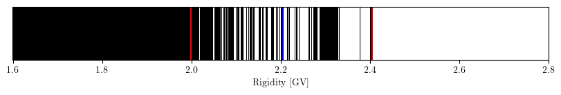
Vertical rigidity barcode for a single location (Moscow example)
This section computes a vertical cutoff barcode for a chosen site:
convert geodetic coordinates (lon/lat/alt) to geocentric Cartesian coordinates,
build a set of particles with different rigidities but identical initial position and vertical direction,
backtrace trajectories and label each rigidity as “allowed” or “forbidden” based on the termination code.
Expected output:
a boolean array (barcode) over rigidity,
numerical estimates of
R_min,R_eff,R_max,a 1D barcode plot with these values marked.
from pyproj import Transformer

lla_to_geo = Transformer.from_crs(
    {"proj": "longlat", "ellps": "WGS84"},
    {"proj": "geocent", "ellps": "WGS84"}
)
def get_vertical_barcode(lon, lat, alt, rigidity_array):
    r = lla_to_geo.transform(lon, lat, alt * 1e3, radians=False)
    v = np.array([
        np.cos(np.deg2rad(lon)) * np.cos(np.deg2rad(lat)),
        np.sin(np.deg2rad(lon)) * np.cos(np.deg2rad(lat)),
        np.sin(np.deg2rad(lat))
    ])
    energy_array = np.sqrt((rigidity_array * 1e3) ** 2 + 938.7 ** 2) - 938.7
    particle = Flux(
        Spectrum=Generators.Spectrums.UserInput(energy=energy_array * Units.MeV),
        Distribution=Generators.Distributions.UserInput(
            R0=np.tile(r, (rigidity_array.size, 1)),
            V0=np.tile(v, (rigidity_array.size, 1))
        ),
        Names="anti_proton",
        Nevents=rigidity_array.size
    )
    simulator = BunemanBorisSimulator(
        Bfield=b_field,
        Region=region,
        Medium=medium,
        Particles=particle,
        InteractNUC=nuclear_interaction,
        UseDecay=use_decay,
        Date=date,
        Step=dt,
        Num=n_steps,
        BreakCondition=break_conditions,
        Save=save,
        Output=output,
        Verbose=verbose
    )
    track_list = simulator()[0]
    barcode = np.array([track["BC"]["WOut"] == 8 for track in track_list])
    return barcode
rigidity_array = np.arange(1.6, 2.801, 0.002)
barcode = get_vertical_barcode(37.32, 55.47, 20, rigidity_array)
def bin_edges_from_centers(x):
    e = np.empty(x.size + 1, dtype=x.dtype)
    e[1:-1] = (x[:-1] + x[1:]) / 2
    e[0] = x[0] - (x[1] - x[0]) / 2
    e[-1] = x[-1] + (x[-1] - x[-2]) / 2
    return e
def get_penumbra_parameters(rigidity_array, barcode):
    rigidity_edges = bin_edges_from_centers(rigidity_array)

    if np.all(barcode):
        return rigidity_edges[0], rigidity_edges[0], rigidity_edges[0]

    if np.all(~barcode):
        return rigidity_edges[-1], rigidity_edges[-1], rigidity_edges[-1]

    idx_true = np.flatnonzero(barcode)
    i_min = idx_true[0]
    r_min = rigidity_edges[i_min]

    idx_false = np.flatnonzero(~barcode)
    i_max = idx_false[-1]
    r_max = rigidity_edges[i_max + 1]

    widths = rigidity_edges[i_min + 1 : i_max + 2] - rigidity_edges[i_min : i_max + 1]
    allowed_width = widths[barcode[i_min : i_max + 1]].sum()
    r_eff = r_max - allowed_width

    return r_min, r_eff, r_max
r_min, r_eff, r_max = get_penumbra_parameters(rigidity_array, barcode)
print('R_min =', r_min, 'GV')
print('R_eff =', r_eff, 'GV')
print('R_max =', r_max, 'GV')
R_min = 1.9990000000000006 GV
R_eff = 2.2049999999999987 GV
R_max = 2.4050000000000007 GV
fig = plt.figure(figsize=(10, 1))
ax = fig.subplots()

rigidity_edges = bin_edges_from_centers(rigidity_array)
ax.pcolormesh(rigidity_edges, np.array([0, 1]), np.array(barcode)[np.newaxis, :], cmap='binary_r', vmin=0, vmax=1)
ax.plot([r_min, r_min], [0, 1], 'r')
ax.plot([r_max, r_max], [0, 1], 'r')
ax.plot([r_eff, r_eff], [0, 1], 'b')
ax.set_yticks([])
ax.set_xlabel('Rigidity [GV]')

plt.show()
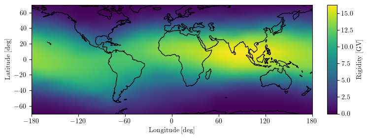
Effective cutoff rigidity map (global scan)
This part demonstrates how to build a global map of the effective vertical cutoff rigidity R_eff:
define a latitude/longitude grid,
compute the barcode and
R_effat each grid node,visualize results on a world map projection.
Expected output: a world map of R_eff (in GV), showing higher cutoffs near the equator and lower cutoffs toward the poles.
# !pip install joblib tqdm_joblib cartopy
from joblib import Parallel, delayed
from tqdm_joblib import tqdm_joblib

import cartopy.crs as ccrs
from mpl_toolkits.axes_grid1 import make_axes_locatable
/home/rustam/Документы/МИФИческое/научка/software/GTsimulation/.venv/lib/python3.12/site-packages/tqdm_joblib/__init__.py:4: TqdmExperimentalWarning: Using `tqdm.autonotebook.tqdm` in notebook mode. Use `tqdm.tqdm` instead to force console mode (e.g. in jupyter console)
  from tqdm.autonotebook import tqdm
lon_grid = np.arange(-180, 161, 20)
lat_grid = np.arange(-70, 71, 10)

r_grid = np.empty((lat_grid.size, lon_grid.size))
Coarse map: fast scan on a wide rigidity grid
To get a quick global overview, we compute R_eff on a coarse rigidity grid (here 0.5 GV step).
With such a step, fine penumbra structure is typically not resolved, but the result is sufficient to estimate typical cutoff levels at different locations.
To reduce runtime, the computation is parallelized over grid points.
Expected output: a coarse global map of R_eff.
rigidity_array = np.arange(0.5, 19.51, 0.5)
def worker(i_lon, i_lat):
    barcode = get_vertical_barcode(lon_grid[i_lon], lat_grid[i_lat], 400, rigidity_array)
    _, r_eff, _ = get_penumbra_parameters(rigidity_array, barcode)
    return i_lon, i_lat, r_eff

tasks = [(i, j) for i in range(lon_grid.size) for j in range(lat_grid.size)]
with tqdm_joblib(total=len(tasks)):
    res = Parallel(n_jobs=-1)(delayed(worker)(i, j) for i, j in tasks)
for i_lon, i_lat, v in res:
    r_grid[i_lat, i_lon] = v
# add the 180° meridian and copy values from the -180° meridian in order to stitch the map seamlessly
lon_grid = np.hstack((lon_grid, 180))
r_grid = np.pad(r_grid, pad_width=((0, 0), (0, 1)), mode="wrap")
fig = plt.figure(figsize=(8, 4))
ax = plt.axes(projection=ccrs.PlateCarree())

pcm = ax.pcolormesh(lon_grid, lat_grid, r_grid, vmin=0)
ax.set_xlim(-180, 180)
ax.set_ylim(-70, 70)
ax.coastlines(resolution="110m", linewidth=1.0, color="black")

ax.set_xticks(np.arange(-180, 181, 60))
ax.set_yticks(np.arange(-60, 61, 20))
ax.set_xlabel('Longitude [deg]')
ax.set_ylabel('Latitude [deg]')

divider = make_axes_locatable(ax)
cax = divider.append_axes("right", size="3.5%", pad=0.3, axes_class=plt.Axes)
fig.colorbar(pcm, cax=cax, label="Rigidity [GV]")

plt.show()

Cutoff values are computed at discrete grid nodes.
In the next cell, the map is rendered with linear interpolation (shading="gouraud") to make the visualization smoother.
fig = plt.figure(figsize=(8, 4))
ax = plt.axes(projection=ccrs.PlateCarree())

pcm = ax.pcolormesh(lon_grid, lat_grid, r_grid, shading="gouraud", vmin=0)
ax.set_xlim(-180, 180)
ax.set_ylim(-70, 70)
ax.coastlines(resolution="110m", linewidth=1.0, color="black")

ax.set_xticks(np.arange(-180, 181, 60))
ax.set_yticks(np.arange(-60, 61, 20))
ax.set_xlabel('Longitude [deg]')
ax.set_ylabel('Latitude [deg]')

divider = make_axes_locatable(ax)
cax = divider.append_axes("right", size="3.5%", pad=0.3, axes_class=plt.Axes)
fig.colorbar(pcm, cax=cax, label="Rigidity [GV]")

plt.show()
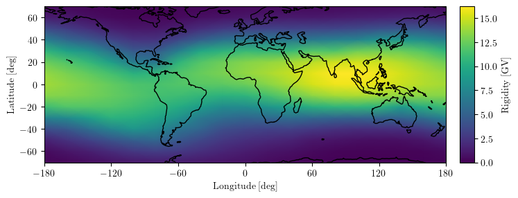
Refined map: local scan around the coarse estimate
This refinement step re-computes R_eff using a finer rigidity step, but only within a narrow interval around the coarse estimate (±1 GV for each grid point).
This approach preserves most of the accuracy benefits while keeping the total runtime manageable.
As before, the computation is parallelized over grid points.
Expected output: a refined global map of R_eff with improved resolution compared to the coarse scan.
# remove the 180° meridian to save computation time
lon_grid = lon_grid[:-1]
r_grid = r_grid[:, :-1]

# copy the previously obtained coarse map
r_grid_base = r_grid.copy()
r_grid = np.zeros_like(r_grid_base)
def worker(i_lon, i_lat):
    rigidity_array = np.arange(r_grid_base[i_lat, i_lon] - 1,
                               r_grid_base[i_lat, i_lon] + 1.01, 0.02)
    rigidity_array = rigidity_array[rigidity_array > 0.001]
    barcode = get_vertical_barcode(lon_grid[i_lon], lat_grid[i_lat], 400, rigidity_array)
    _, r_eff, _ = get_penumbra_parameters(rigidity_array, barcode)
    return i_lon, i_lat, r_eff

with tqdm_joblib(total=len(tasks)):
    res = Parallel(n_jobs=-1)(delayed(worker)(i, j) for i, j in tasks)
for i_lon, i_lat, v in res:
    r_grid[i_lat, i_lon] = v
# add the 180° meridian and copy values from the -180° meridian in order to stitch the map seamlessly
lon_grid = np.hstack((lon_grid, 180))
r_grid = np.pad(r_grid, pad_width=((0, 0), (0, 1)), mode="wrap")
fig = plt.figure(figsize=(8, 4))
ax = plt.axes(projection=ccrs.PlateCarree())

pcm = ax.pcolormesh(lon_grid, lat_grid, r_grid, vmin=0)
ax.set_xlim(-180, 180)
ax.set_ylim(-70, 70)
ax.coastlines(resolution="110m", linewidth=1.0, color="black")

ax.set_xticks(np.arange(-180, 181, 60))
ax.set_yticks(np.arange(-60, 61, 20))
ax.set_xlabel('Longitude [deg]')
ax.set_ylabel('Latitude [deg]')

divider = make_axes_locatable(ax)
cax = divider.append_axes("right", size="3.5%", pad=0.3, axes_class=plt.Axes)
fig.colorbar(pcm, cax=cax, label="Rigidity [GV]")

plt.show()

fig = plt.figure(figsize=(8, 4))
ax = plt.axes(projection=ccrs.PlateCarree())

pcm = ax.pcolormesh(lon_grid, lat_grid, r_grid, shading="gouraud", vmin=0)
ax.set_xlim(-180, 180)
ax.set_ylim(-70, 70)
ax.coastlines(resolution="110m", linewidth=1.0, color="black")

ax.set_xticks(np.arange(-180, 181, 60))
ax.set_yticks(np.arange(-60, 61, 20))
ax.set_xlabel('Longitude [deg]')
ax.set_ylabel('Latitude [deg]')

divider = make_axes_locatable(ax)
cax = divider.append_axes("right", size="3.5%", pad=0.2, axes_class=plt.Axes)
fig.colorbar(pcm, cax=cax, label="Rigidity [GV]")

plt.show()
Potential ways to improve accuracy and resolve finer penumbra structure:
Decrease the integration time step (e.g., down to 1e-6 s).
Use a finer rigidity step (e.g., 0.001 GV) in the barcode scan.
Increase the latitude/longitude grid resolution.